Generalizing Secret Santa with integer programming in Julia

Paul Butler – December 10, 2022

You might know Secret Santa as the gifting game where each person in a group is assigned another person in the group to give a gift to.

For three years in a row, I’ve organized a post card exchange for plotter enthusiasts called #ptpx, which I think of as a sort of “generalized Secret Santa”. Instead of just sending and receiving one gift, participants choose how many postcards they’d like to make and send.

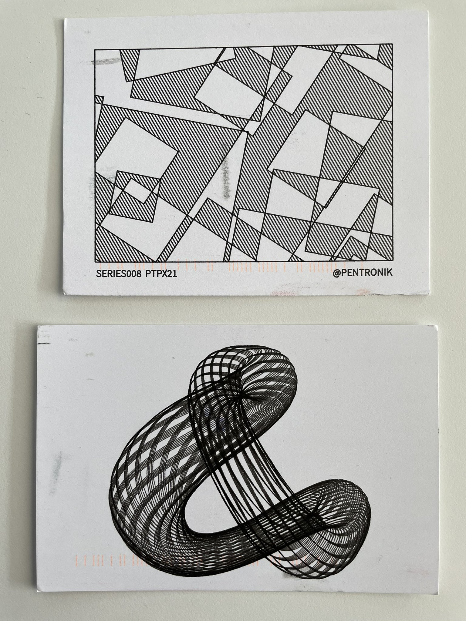
To give you an idea, here are some cards I received last year from @pentronik and @aldernero:

You can think of any gift exchange as a directed graph, with each node representing a participant, and edges going from senders to receivers. A traditional, 1:1 Secret Santa could be organized by shuffling all of the participants, and having each send a gift to the next person in order (wrapping around at the end).

The generalized variant of Secret Santa has no such trivial construction, so instead I’ve turned to integer programming.

Integer programming, and optimization in general, can seem a bit scary to people (like myself) who have no formal background in it, so I wanted to demystify it by showing how I use it to solve a real-world problem.

Constraints

We’ve established that we need to generate a graph, so let’s formalize the constraints in terms of a graph:

Each participant sends as many cards as they signed up for. This is a constraint on the out-degree of each node.
Each participant receives as many cards as they signed up for. This is a constraint on the in-degree of each node.
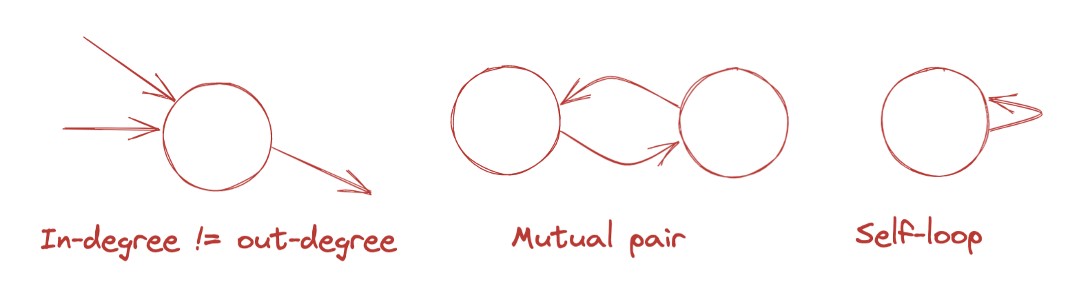
No participant sends a card to themselves. There are no self-loops.
To keep things interesting, there are no direct mutual exchanges in which a participant both sends and receives a card from the same other participant. The graph has a minimum girth of three.

Here’s a diagram of some graphs these constraints prevent:

Matrix form

A directed graph can be expressed as a square matrix A in which the i^th node corresponds to both the i^th row and the i^th column. The matrix cell A_jk contains a 1 if the corresponding graph node j has an out-edge to graph node k; otherwise it contains a 0.

Our constraints can be translated into this matrix form.

Each participant sends as many cards as they signed up for. The sums of each row equal (element-wise) the cards to be sent by each participant.
Each participant receives as many cards as they signed up for. The sum of each column (element-wise) equals the number of cards to be received by each participant.
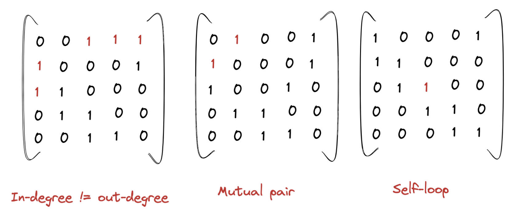
No participant sends a card to themselves. The diagonal entries of the matrix are all zero.
No mutual exchanges. For all nodes j and k, the entry at A_jk and A_kj are mutually exclusive.

Here are some examples of adjacency matrices that violate these constraints:

Linear optimization

For the purpose of generating the adjacency matrix, the only information we need is an array with the desired number of cards for each participant. For example, if we have five participants who want to send three cards and four participants who want to send two cards, we could represent that as:

node_degrees = [3, 3, 3, 3, 3, 2, 2, 2, 2]

We could order these however we want, as long as we preserve a mapping so that we know which participant each entry refers to.

Our job is then take a list in this form, and return an adjacency matrix that satisfies the four properties mentioned above.

I’ve chosen to use Julia for this, because of its excellent JuMP optimization library.

JuMP does not implement a solver itself, but instead provides a friendly Julia-based interface that can map to a variety of solvers which must be installed separately.

There are different types of solvers which support different types of constraints. Because my constraints aren’t very fancy, and I don’t know much about this stuff, I didn’t put too much thought into selecting a solver. I picked SCIP because it was free and easy to install.

JuMP is fairly straightforward to use. The steps are:

1: Create a model object and select an optimizer.

model = Model(SCIP.Optimizer)

2: Define the variables you want to optimize over.

In our case, this means one binary variable for each cell in the adjacency matrix.

N = length(node_degrees)

@variable(model, x[s=1:N, r=1:N], Bin)

JuMP uses Julia macros (which start with @) to create a sort of domain-specific language for specifying models within Julia.

In this case, I’m telling it to create a variable called x, attached to the model we just created, representing an N-by-N matrix of binary (Bin) values. We’ve defined N to be the number of participants in the exchange.

3: Define the constraints you want the solution to satisfy.

@constraint(model,
    cards_sent[i=1:N], sum(x[i,:]) == node_degrees[i])

This creates an array of N constraints called cards_sent that ensures that the sum of the i^th row is equal to the number of cards that the i^th participant signed up to send.

@constraint(model,
    cards_received[i=1:N], sum(x[:,i]) == node_degrees[i])

Similarly, this creates an array of N constraints called cards_received that ensures that the sum of the i^th column is equal to the number of cards that the i^th participant should receive.

@constraint(model, no_mutual_exchange[i=1:N,j=1:i], x[i,j] + x[j,i] <= 1)

This creates more constraints called no_mutual_exchange which ensure that each participant can either be a sender or receiver to a given other participant, but not both.

We could also specify a condition to explicitly prohibit self-loops:

@constraint(model, no_self_loop[i=1:N], x[i,i] == 0)

But we don’t actually need to. A self-loop would be considered a mutual exchange by the definition we used above, since if x[k, k] == 1, x[k, k] + x[k, k] > 1 in violation of no_mutual_exchange[k, k].

4: Optionally, define an objective you want the solver to maximize.

We can skip this, because we don’t have an objective to optimize for.

5: Run the solver.

Tell JuMP that you’re done specifying the model and ready to run it, then wait and retrieve the result.

optimize!(model)

This attempts to find a value of the variable(s) in question that satisfy the constraints and (if there is one) maximize the objective.

result = JuMP.value.(x) .== 1.0

Finally, we pull the resulting value assigned to the variable. Even though we declared x as binary, JuMP returns it as a Matrix{Float64}, so we use element-wise equality with 1.0 to get back a BitMatrix.

Here’s an example value of result for the example input above, [3, 3, 3, 3, 3, 2, 2, 2, 2]:

 0  0  0  0  0  1  0  1  1
 1  0  0  0  0  1  0  1  0
 1  1  0  0  0  0  0  0  1
 1  1  1  0  0  0  0  0  0
 0  1  1  1  0  0  0  0  0
 0  0  1  0  1  0  0  0  0
 0  0  0  1  1  0  0  0  0
 0  0  0  0  1  0  1  0  0
 0  0  0  1  0  0  1  0  0

We can verify by hand that:

The first five columns and five rows sum to 3, and the remaining rows and columns sum to 2, matching the desired number of cards sent/received in the input vector.
There are no 1s along the diagonal, so nobody sends a card to themselves.

It’s harder by eyeball to ensure that there are no mutual exchanges, but it’s a one-liner to test:

result .& result'

This does an element-wise AND between the matrix and its transpose. This will leave a 1 for every exchange pair that is mutual, so if the result is a zero matrix (as it is in this case), there are no mutual exchanges.

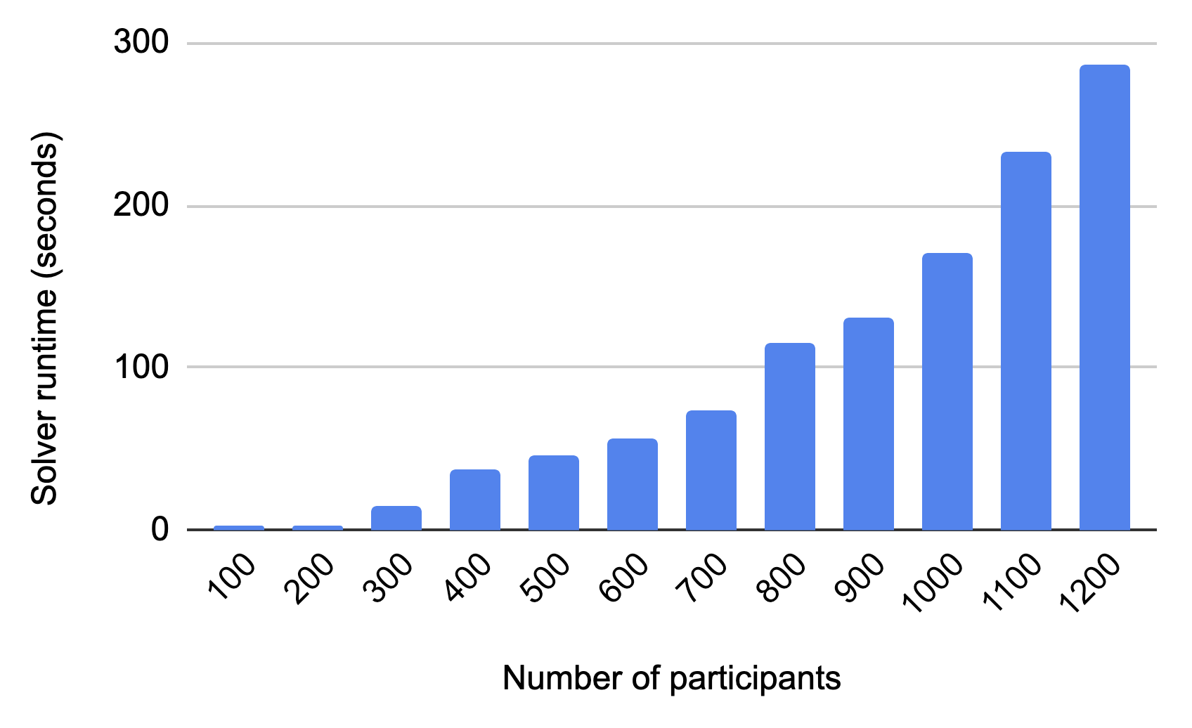
Performance

I’m not sure what the runtime complexity of SCIP’s solving function is, but I know the overall algorithm is at least O(n^2) on the number of participants n, because the size of the output matrix is n-by-n.

The exchange I organized in 2020 had 22 participants. In 2021, we had 40. This year, the number grew to 76. So I’ve been wondering, how big would it have to get before I can’t use my program to solve it?

To answer this, I generated simulated exchanges with different numbers of participants. Although the runtime is worse than linear, I can still solve exchanges with up to 1,200 participants in under five minutes on my M1 mac.